SQL Server 2008: Spatial indexes

Note: all images in this post are taken from November CTP Books Online

There are two kinds of spatial data that 2008 supports – planar (i.e. points, lines, polygons on a single 2-D plane) and geodetic (i.e. points, lines, polygons on a geodetic ellipsoid – for example, the Earth). These are presented in SQL as geometry and geography data respectively. A common operation that’s performed on spatial data is comparing two spatial values to see if they intersect at all. Now, this is a complicated calculation, which gets more computationally expensive as the complexity of the spatial values increase. Given a problem of ‘which spatial values in this table does this spatial value X intersect with’, it would be great to have some way of quickly pruning out spatial values in the table that cannot possibly intersect with X, and so avoid doing the expensive calculation for them. Enter spatial indexes.

Here’s the basic idea behind a spatial index:

• 
  
  A plane is broken up into a grid of cells.
  
  
• 
  
  Each spatial value is evaluated to see which cells in the grid it intersects with
  
  
• 
  
  The list of cells is stored along with the primary key of the table row that the spatial value is part of
  
  
• 
  
  Comparing two spatial values for intersection is a matter of comparing the list of grid cells – if there are no matching cells, the spatial values do not intersect, and there’s no need to do the expensive intersection calculation

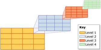
In practice its a bit more complicated. For planar data (i.e. the geometry data type), you need to define a bounding box (i.e. 4 corner points that define a rectangle of space in which you’re interested on the 2-D plane). That bounding box on the plane will be broken down into a grid of cells. The top-level grid can be up to 16×16, giving 256 cells. The next level of granularity breaks each of those top-level grid cells into a further grid, again up to 16×16. So now there could be (16×16) x (16×16) cells in the grid – or 65536 cells. This obviously allows a more exact description of a spatial value in the list of cells. And so on and so on. There are actually 4 levels of grid that the bounding box is broken up into – and each can be 16×16, for a possible total of 16⁸ or 4 billion cells. The picture below illustrates this with a grid size of 4×4 at each level.

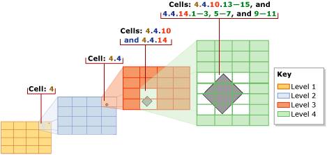
The bounding box and the size of the grid at each level are specified when the spatial index is created, as well as the maximum number of matching grid cells to store in the spatial index per spatial value – to a max of 8192. Once the bounding box has been decomposed into the various levels of grid, each value in the spatial column is evaluated against the grid. The value is first decomposed against the first level grid. If the number of cells it matches is less than the max per spatial value, the decomposition then moves to the second level grid. This decomposition continues until the maximum number of matching grid cells is reached. If the max is reached while processing a deeper level for a cell, (e.g. in the middle of processing the 2^nd level grid of 4×4 for cell #13 in the 1^st level), the deeper level matches are thrown away and only the coarser granularity matching cell is stored (e.g. continuing that example, the 2^nd level grid matches are discarded and only cell #13 in the 1^st level will be stored). The picture below helps to illustrate this.

So, each geometric spatial value is approximated in the spatial index by a list of matching cells in the defined bounding box. As there is a limit to the number of matching cells that can be stored in the approximation, it is an optimistic representation. This means that if two values are compared using the approximations, there will be no false negatives, as the approximations map a larger space than the actual spatial values. There can, however, be false positives. A false (or real) positive means the spatial values need to then be compared using the complex, computationally expensive intersection algorithm using the actual spatial values. So again, the spatial index serves as a way of pruning out the need to run the expensive algorithm.

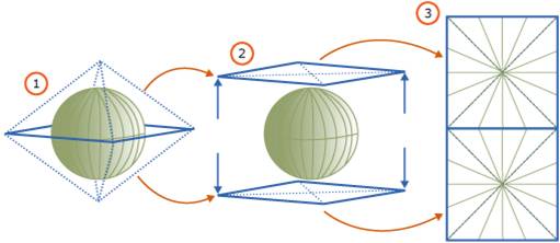
The algorithm is very similar for geodetic data (i.e. the geography data type), however there’s no bounding box. Instead, the entire geodetic ellipsoid is projected onto a 2-D plane and then the grid decomposition algorithm is applied to that plane in exactly the same way as for planar data. The picture below describes how the projection is done.

You may have already realized that the effectiveness of the spatial index in pruning is directly proportional to how exactly the approximations in the index actually describe the spatial values. In other words, the higher the number of grid cells at each level, and the higher the number of grid cell matches that are stored per spatial value in the index, the better the index is at pruning. More exact approximations require storing more matching grid cells at deeper granularities – i.e. taking MORE SPACE. Creating a more exact spatial index takes more space.

With all that in mind, the interesting thing for DBAs here is that there’s a trade-off between CPU use to do the real intersection algorithm and spatial index size to use in pruning calls to the algorithm. It’s too early to know what best practices there are – but I’ll blog them as I here about them.